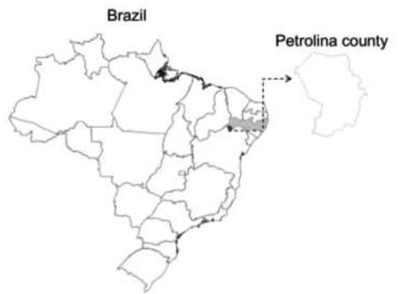
Figure 1. Location of the experiment, Petrolina county, Pernambuco state, Brazil
Figura 1. Localização do experimento, Petrolina, Pernambuco, Brasil
GÉNESIS, CLASIFICACIÓN, CARTOGRAFÍA Y MINERALOGÍA DE SUELOS
Soil mapping quality for site-specific management in fruit fields in the semiarid region of Brazil
Qualidade do mapeamento do solo para manejo específico em frutíferas na região semiárida do Brasil
Marcos Sales Rodrigues*1; David Castro Alves1; Jailson Cavalcante Cunha1; Júlio César Ferreira de Melo Júnior1; Augusto Miguel Nascimento Lima1; Aíris Layanne Ferreira Lira1; Filipe Bernard; Kátia Araújo Silva1
1 Universidade Federal do Vale do São Francisco, Brasil
* Autor de contacto: marcos.rodrigues@univasf.edu.br
Recibido: 28/1/2019
Recibido con revisiones: 14/5/2019
Aceptado: 15/5/2019
ABSTRACT
Soil mapping is an important technique to apply site-specific management in fruit fields. Therefore, aims of this
study were to evaluate soil sampling methods and the use of interpolator techniques in the quality of soil texture
maps in a mango field; and to evaluate the efficiency of the use of independent data set in the validation of maps
process. The experiment was in a 3.3 ha mango commercial orchard in the semiarid region of Brazil. The samples
were collected following a regular grid containing 119 georeferenced spaced 14 x 20 m points, in addition
to five micro-grids each containing six spaced 7 x 10 m points. To obtain an independent dataset for the maps
validation, 40 random samples were performed. Soil texture was determined. Geostatistic and deterministic
interpolation techniques were performed. Cross-validation method with internal and independent dataset was
performed to validate the maps. All variables showed a strong spatial dependence. Kriging was slightly better
than the deterministic interpolation techniques, showing root mean square errors of 2,40%; 2,84%; and 2,59%
for clay, sand, and silt content, respectively. The use of micro-grid did not reduce the errors of the maps. The
independent dataset showed efficient to validate soil texture maps since its values represent the real accuracy.
Keywords: Cross-validation, interpolation methods, geostatistics, soil texture.
RESUMO
O mapeamento do solo é uma técnica importante para aplicar manejo específico em frutíferas. Portanto, os
objetivos deste estudo foram avaliar métodos de amostragem do solo e o uso de técnicas de interpoladores na
qualidade dos mapas de textura do solo em uma área de manga e avaliar a eficiência do uso de conjuntos independentes
de dados no processo de validação de mapas. O experimento foi realizado em um pomar comercial
de 3,3 ha de manga, na região semiárida do Brasil. As amostras foram coletadas seguindo uma malha regular
contendo 119 pontos georreferenciados espaçados de 14 x 20 m, além de cinco micro-malhas contendo cada
uma seis pontos espaçados de 7 x 10 m. Para obter um conjunto de dados independente para a validação dos
mapas, foram realizadas 40 amostras aleatórias. A textura do solo foi determinada. Técnicas de interpolação
geoestatística e determinística foram realizadas. O método de validação cruzada com conjunto de dados interno
e independente foi realizado para validar os mapas. Todas as variáveis mostraram forte dependência espacial.
A Krigagem foi um pouco melhor do que as técnicas de interpolação determinística, mostrando erros de raiz
quadrada média de 2,40%; 2,84%; e 2,59% para argila, areia e silte, respectivamente. O uso da micro-malha
não reduziu os erros dos mapas. O conjunto de dados independente mostrou-se eficiente para validar mapas de
textura do solo, uma vez que seus valores representam a precisão real.
Palavras-chave: Validação cruzada, técnicas de interpolação, geoestatística, textura do solo.
INTRODUCTION
Mapping soil properties is a preliminary step towards decision making such as identification of management zones and apply site-specific management (Bilgili, 2013). Although digital soil mapping has been increasing around the world, including Brazil, little attention is paid to the quality of the maps that are produced (Brus et al., 2011). In addition, there are no studies about this theme for irrigation areas in the semiarid region of Brazil.
Several factors are related to soil map quality, however, three can be highlighted, which are: 1) the number of samples collected (Bottega et al., 2014) and sampling method (Yates et al., 2008), 2) interpolation method (deterministic or geostatistical) (Bier & Souza, 2017) and 3) method of map validation (cross-validation with internal dataset or with independent dataset) (Brus et al., 2011).
The most common sample design adopted for soil mapping is the regular grid. However, when there is a structure with a range shorter than the sampling interval, there is an increase in the nugget effect in semivariograms and, consequently, an increase in map error. One commonly used strategy to reduce this error is the use of refined grids with smaller spacing within the main grid (Barbosa et al., 2012; Montanari et al., 2012; Dalchiavon et al., 2014).
The spatial variability of soil properties is often assessed with data interpolation (Silva et al., 2017), thus, selecting a proper spatial interpolation method is important, since different methods of interpolation can lead to different results (Li & Heap, 2011).
In this context, one question should be answered: how to choose the most quality map? An option is leave-one-out cross-validation method. This method involves consecutively removing a data point, interpolating the value from the remaining observations and comparing the predicted value with the measured value (Xie et al., 2011), and then the prediction error is computed. However, the validation of the map is performed using the data from itself data set. According to Brus et al. (2011), the accuracy thus obtained, referred to as the internal accuracy, often over-estimates the actual accuracy. Therefore, predictions are preferably compared with independent dataset not used in the modeling.
Since, the soil textural distribution information is important for planning agriculture crop production, irrigation management, hydrological analysis and soil characteristics determination (Deshmukh & Aher, 2014), this variable was used in this work.
Therefore, aims of this study were to evaluate (1) soil sampling methods and (2) the use of deterministic and geostatistics interpolators in the quality of soil texture maps in a fruit field in the semi-arid region of Brazil; and to evaluate (3) the efficiency of the use of independent dataset in the validation of maps process.
MATERIALS AND METHODS
Site description
This experiment was conducted in the Nilo Coelho irrigated perimeter, Petrolina county, Pernambuco state, northeastern Brazil (9º19’36.47” S, 40º36’40.92” W, 405 m a.s.l.) (Figure 1). The climate of the region, according to the Köppen classification, is of the ‘hot semi-arid’ (Bsh) type, characterized by high temperatures (average 26°C), low humidity, high evaporation rates, and especially marked by the scarcity and irregularity in rainfall distribution (400 mm). The soil of the experimental area was classified as Yellow Argisol (Ultisol - American classification Soil Taxonomy). The experimental area (3.3 ha) was a mango commercial orchard (cv. Kent) spaced 7 x 5 m and irrigated by micro-sprinkler.
Figure 1. Location of the experiment, Petrolina county,
Pernambuco state, Brazil
Figura 1. Localização do experimento, Petrolina, Pernambuco,
Brasil
Soil sampling and laboratory analysis
The samples were collected following a regular grid containing 119 georeferenced spaced 14 x 20 m points, where the distance was determined based on the plant spacing. In addition to five micro-grids, each containing six spaced 7 x 10 m points. To obtain an independent data set for the maps validation, 40 random samples were performed (Figure 2). For the three data sets the coordinates were added using a Google Earth® image of the area.
Soil samples were collected at each georeferenced point in the canopy region of the mango trees using a Dutch auger at the layers of 0-0.2 and 0.2-0.4 m depth. Samples were dried at room temperature and passed through a sieve with apertures of 2.0 mm. Each soil sample was analyzed for particle size (pipette method) to obtain the clay, sand and silt fractions according to the methodology described by Donagema et al. (2011).
Preliminary statistical analysis
Descriptive statistical analysis (mean, maximum, minimum, standard deviation, coefficient of variation - CV, coefficient of asymmetry and kurtosis) were calculated. To test the hypothesis of normality, the Ryan-Joiner test was conducted.
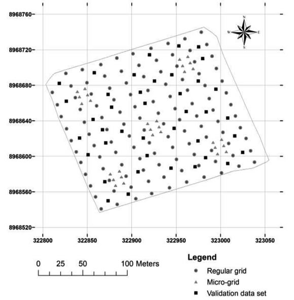
Figure 2. Sampling scheme for soil attributes
in an irrigated mango orchard in the semi-arid
region of Brazil (Datum WGS 1984, UTM Zone
24 South)
Figura 2. Esquema de amostragem para atributos
do solo em pomar de mangueira irrigada na
região semiárida do Brasil (Datum WGS 1984,
Zona UTM 24 Sul)
Geostatistical analysis and mapping
Spatial dependence of samples was estimated using experimental semivariograms and theoretical mathematics models (Oliver & Webster, 2014). In this work the most common semivariogram models were tested, which are: spherical, exponential, and Gaussian model (Zůvala et al., 2016).
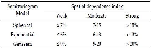
The spatial dependence index (SDI) proposed by Seidel & Oliveira (2016) was used to determine the degree of spatial variability. This index takes into account the semivariogram model, the nugget effect, contribution (partial sill), range and, the maximum distance between sampled points (240 m for the present study). The classification can be found in Table 1.
Table 1. Spatial dependence index classification for soil
attributes suggested by Seidel & Oliveira (2016).
Tabela 1. Classificação do índice de dependência espacial para
atributos do solo sugerida por Seidel & Oliveira (2016).
After the estimation of experimental semivariograms and adjustment of theoretical models, the data were interpolated using ordinary kriging, generating soft maps. Kriging is a generic term for a range of least squares methods to provide the best linear unbiased predictions, best in the sense of minimum variance (Oliver & Webster, 2014).
In addition, three deterministic interpolation techniques were performed which were: Inverse distance weighting (IDW), Radial basis functions (RBF) and Local Polynomial interpolation (LPI).
IDW interpolation technique is based on the premise that the predictions are a linear combination of available data. Power equal to 2 was used for IDW. RBF is conceptually similar to fitting a rubber membrane through the measured sample values while minimizing the total curvature of the surface. Spline with Tension was the kernel function chosen for RBF. LPI is a process of finding a formula (often a polynomial) whose graph will pass through a given set of points. A complete explanation of these interpolation techniques can be found in Xie et al. (2011). All maps were produced using ArcGIS 10.6 Student License.
Cross-validation analysis
Cross-validation method was used for verifying the quality of the maps using only the regular grid, and the regular grid plus micro-grids in each interpolation technique tested. Three indices were used to determine the best sampling design (regular grid and regular grid + micro-grids) and the best interpolation techniques which were: Mean Error (ME), Mean Square Error (MSE) and, Root Mean Square Error (RMSE).
The ME is defined by (Eq. 1):
where vi was the difference between the predicted value and observed value at location si, i 1,…, nv, and nv was the number of values in the check data set.
The MSE was the sum of accuracy and precision. It was defined in Eq. (2):
where vi2 was the difference between the square of predicted value and observed value at location si, i 1,…, nv, and nv was the number of values in the check data set. The RMSE was defined as Eq. (3) and it represents the error in the variable unit.
Smaller ME, MSE and RMSE values indicate fewer errors.
The prediction power was estimated by the amount of variance explained (AVE) it is defined as (Eq. 4) (Angeline et al., 2017):
where yi is the i-th measurement of the target variable, ŷi is the corresponding predicted value, ȳ is the mean and n is the number of observations.
In addition, cross-validation was also performed using independent dataset obtained from de 40 samples to test the external accuracy (Brus et al., 2011).
RESULTS AND DISCUSSION
Descriptive statistical results
Based on the mean values, the soil was classified as a sandy loam for the layers of 0-0.2 and 0.2-0.4 m depth. The minimum, maximum, and, standard deviation values indicate that there is high variability in the study field, mainly for clay and silt content (Table 2). Based on the coefficient of variation (CV) classification (Pimentel-Gomes & Garcia, 2002), the sand content showed low variation (CV < 10%), whereas clay and silt content showed high variation (CV = 20-30%), except for clay content at the layer of 0-0.2 m depth using the regular grid plus micro-grid which showed very high variation (CV > 30%) (Table 2). Similar results were found by Rodrigues et al. (2018) in mango field under Alfisol in the semiarid region of Brazil, where sand content was classified as low variation and silt and clay content as a very high variation.
Table 2. Descriptive statistics of soil texture (%) at the layers of 0-0.2 m and 0.2-0.4 depth in an irrigated mango field in the semi-arid
region, Brazil
Tabela 2. Estatística descritiva da textura do solo (%) nas camadas de 0-0,2 m e 0,2-0,4 de profundizado em mangueira irrigada na
região semiárida Brasil
St. dev. = standard deviation; Var. = Variation; Asy. = Asymmetry; Kur. = Kurtosis; p-value (0.05) of normality test; Normality = Ryan-Joiner normality test; Non-N
= Non-normal
St. dev. = desvio padrão; Var. = Variação; Asy. = Assimetria; Kur. = Curtose; p-value (0,05) do teste de normalidade; Normalidade = teste de normalidade de Ryan-
Joiner; Non-N = não-normal
Rodrigues et al. (2015) in an irrigated guava field in the semi-arid region of Brazil verified that, even in a small field, soil texture can vary considerably. Therefore, wrong decisions could be made when the management of water and fertilizer is defined by average values.
The clay and silt fractions showed normal distribution data, excepted for the silt fraction at the layer of 0.2-0.4 m depth using the regular grid plus the micro-grid. On the other hand, the sand fraction showed non-normal distribution data (Table 2). Even though Li & Heap (2011) have reported that normality of data may affect the performance of spatial interpolation methods, Wu et al. (2006) demonstrated that the quality of maps from normal and non-normal data set was very small when high asymmetry and kurtosis are not observed, as verified in the present study (Table 2). Additionally, Yamamoto (2007) states that when the transformed data is used, it is necessary a back-transformation and in this case, kriging estimates are biased because the nonbias term is totally dependent on a semivariogram model. Therefore, data transformation was not performed.
Spatial structure and sample design
All studied variables at both layers showed spatial dependence. The highest range (250 m) was observed for the sand content at the layer of 0-0.2 m depth when the micro-grid was not used and at the layer of 0.2-0.4 m depth when the micro- grid was used, whereas the lowest range (56 m) was observed for the clay content at the layer of 0.2-0.4 m depth using the micro-grids data (Table 3). The spatial dependence was strong for all texture fraction at the layer of 0-0.2 m depth. On the other hand, only sand content showed strong spatial dependence at the layer of 0.2-0.4 m depth regardless of the sampling design (with or without micro-grids).
Table 3. Variogram model parameters of soil texture (%) at the layers of 0-0.2 m and 0.2-0.4 depth in an irrigated mango field in the
semi-arid region, Brazil
Tabela 3. Parâmetros do modelo de variograma da textura do solo (%) nas camadas de 0-0,2 m e 0,2-0,4 de profundidade em
mangueira irrigada na região semiárida Brasil
SDI = spatial dependence index (Seidel & Oliveira, 2016)
SDI = índice de dependência espacial (Seidel & Oliveira, 2016)
Similar results were found by Bottega et al. (2014), which verified strong dependence for the texture fractions of an Oxisol under a no-tillage system in Sidrolândia county, Mato Grosso do Sul state, Brazil. Strong spatial dependence for soil texture is expected since it is a very stable soil attribute because it is more related to parent material and pedogenetic processes than to anthropogenic processes.
The use of micro-grid decreased the nugget effect for sand and silt content at both studied layers (Table 3). The nugget effect can be attributed to measurement errors or spatial sources of variation at distances smaller than the sampling interval or both. Variation at microscales smaller than the sampling distances will appear as part of the nugget effect (Carrasco, 2010). The micro-grid has been used with the purpose of detecting spatial dependence ranges for spaces smaller than the principal grid spacing (Barbosa et al., 2012; Montanari et al., 2012; Dalchiavon et al., 2014), thus, the nugget effect may be reduced. This could contribute to the reduction of interpolation error when using a stochastic interpolator such as Kriging. However, observing the map quality indices, no significant errors reduction was verified in Kriging maps. Therefore, for the purpose of saving financial resources, the use of micro-grids for soil texture mapping would not be justified, since the improvements in the maps have not been proven. This possibly occurred because the spacing and the density of the sample were enough to capture the spatial dependence of the area for the soil texture, even in small scale, thus, the micro-grid was not necessary. However, it is important to highlight that in case that greater part of the nugget effect is related to measurement errors in the data, it may limit the improve of map accuracy.
Interpolation techniques
The Kriging technique showed the smaller ME (Mean Error) values among the interpolation methods tested (Table 4). ME is used for determining the degree of bias in the estimates, however, according to Li & Heap (2011) it should be used cautiously as an indicator of accuracy because negative and positive estimates counteract each other, and resultant bias tends to be lower than the actual error. Therefore, the analysis of soil map quality should consider other indices such as RMSE (Root mean square error) and AVE (Amount of variance explained).
Based on the three indices of quality of maps the kriging presented a slightly better performance in relation to the other interpolators (Table 4). The accuracy of soil texture maps showing the following order Kriging>LPI>IDW>RBF. As reported by Li & Heap (2011), in most of the studies comparing interpolation methods in environmental sciences, stochastic techniques (geostatistical) showed better results than deterministic techniques.
While the deterministic methods calculate the unknown values based on parameters that control either the extent of the similarity of values (e.g., IDW) or the degree of smoothing of the surface (e.g., RBF), the stochastic methods (e.g., Kriging) assume that at least part of the spatial variation of natural phenomena can be modeled by random processes with spatial autocorrelation (Dai et al., 2014). Therefore, Kriging is considered the best linear unbiased estimator in the sense that it minimizes the variance of the estimation error (Oliver & Webster, 2014).
Independent dataset
The independent dataset cross-validation indices values (Table 5) were higher than those from the internal dataset (Table 4). This was more prominent in the ME, but the RMSE values, which represent the error in the variable unit, was only slightly greater. These results are expected due to the number of observations used for cross-validation with internal data set (all observation) is greater than the independent dataset (40 samples).
Table 4. Cross-validation indices using internal data set of soil texture (%) at the layers of 0-0.2 m and 0.2-0.4 depth in an irrigated
mango field in the semi-arid region, Brazil
Tabela 4. Índices de validação cruzada usando o conjunto de dados internos da textura do solo (%) nas camadas de 0-0,2 m e 0,2-0,4
de profundidade em mangueira irrigada na região semiárida Brasil
IDW = Inverse distance weighting; RBF = Radial basis functions; LPI = Local Polynomial interpolation. ME = Mean error; AVE = Amount of variance
explained; RMSE = Root mean square error
IDW = ponderação do inverso da distância; RBF = funções de base radial; LPI = interpolação polinomial local. ME = erro médio; AVE = quantidade de variância
explicada; RMSE = raiz quadrática média do error
Table 5. Cross-validation indices using independent data set of soil texture (%) at the layers of 0-0.2 m and 0.2-0.4 depth in an
irrigated mango field in the semi-arid region, Brazil
Tabela 5. Índices de validação cruzada usando o conjunto de dados independentes da textura do solo (%) nas camadas de 0-0,2 m e
0,2-0,4 de profundidade em mangueira irrigada na região semiárida Brasil
IDW = Inverse distance weighting; RBF = Radial basis functions; LPI = Local Polynomial interpolation. ME = Mean error; AVE = Amount of variance
explained; RMSE = Root mean square error
IDW = ponderação do inverso da distância; RBF = funções de base radial; LPI = interpolação polinomial local. ME = erro médio; AVE = quantidade de
variância explicada; RMSE = raiz quadrática média do erro
Although the cross-validation performed with an internal data set has presented smaller values (Table 4), these values represent the internal accuracy and the results may be biased (Brus et al., 2011). Mueller et al. (2001) studying map quality for site-specific fertility management in Clinton County, Michigan, verified that cross-validation with an independent dataset directly estimates the spatial uncertainty, as validation points are located randomly throughout the field. Thus, they concluded that cross-validation with independent data was superior to cross-validation with internal dataset as a basis for measuring map quality.
However, the use of independent dataset may increase sampling and analysis cost, since it increases the number of soil samples. Thus, the development of sensors that evaluate soil properties is fundamentally important, since these sensors can increase the number of samples, consequently, increase the soil mapping quality and decrease the soil sampling cost. Examples of sensors which can predict soil texture can found in works developed by Piikki et al. (2013) and Wetterlind et al. (2015). In addition, there are sensors for other soil properties such as the portable X-ray fluorescence spectrometer, which is useful for determining the total content of chemical elements in soils (Udeigwe et al. 2015), the soil magnetic susceptibility sensor which can be used to estimate soil chemical elements (Jakšík et al. 2016) and soil texture and the apparent electrical conductivity of soil, which has been used to estimate and map the spatial variability of some soil properties (Grubbs et al. 2018).
Based on the data, we recommend the production of the maps of soil texture using Kriging interpolation without the micro-grids, as shown in Figure 3.
Figure 3. Soil texture maps of an irrigated mango field in the semi-arid region, Brazil, using the data set without micro-grids
interpolated by Kriging
Figura 3. Mapas de textura do solo em área de mangueira irrigada na região semiárida, Brasil, usando os conjuntos de dados sem
micro-malhas interpoladas por Krigagem
CONCLUSIONS
The use of micro-grid did not reduce the errors of the maps. Therefore, for the present study, micro- grids were not necessary for soil texture mapping. Kriging presented a slightly better performance in relation to the other interpolators. Since the errors obtained with the independent dataset represent the real accuracy, it should be preferred compared to the internal dataset for mapping validation.
ACKNOWLEDGMENT
We would like to thank Mr. Cleiton Nogueira Martins from Agropecuária J. Martins farm form allowing the use of the experiment area. To CNPq (National Council of Scientific Researchers) for providing a scholarship to the second author.
REFERENCES
1. Angelini, ME; GBM Heuvelink & B Kempen. 2017. Multivariate mapping of soil with structural equation modelling. European Journal of Soil Science 68(5): 575-591.
2. Barbosa CEM.; S Ferrari; MP Carvalho; PRF Picoli; MC Cavallini; CGS Benett & DMAD Santos. 2012. Inter-relação da produtividade de madeira do pinus com atributos físico-químicos de um latossolo do cerrado brasileiro. Revista Árvore 36(1): 25-35.
3. Bier VA & EG Souza. 2017. Interpolation selection index for delineation of thematic maps. Computers and Electronics in Agriculture 136: 202-209.
4. Bilgili A. 2013. Spatial assessment of soil salinity in the Harran Plain using multiple kriging techniques. Environmental Monitoring and Assessment 185(1): 777-795.
5. Bottega EL; DM Queiroz; FAC Pinto & NT Santos. 2014. The use of different sampling grids in determining the variability of soil physical attributes of Oxisol. Comunicata Scientiae 5(2): 131-139.
6. Brus DJ; B Kempen & GBM Heuvelink. 2011. Sampling for validation of digital soil maps. European Journal of Soil Science 62(3): 394-407.
7. Carrasco PC. 2010. Nugget effect, artificial or natural? Journal of the Southern African Institute of Mining and Metallurgy 110: 299-305.
8. Dai F; Q Zhou; Z Lv; X Wang & G Liu. 2014. Spatial prediction of soil organic matter content integrating artificial neural network and ordinary kriging in Tibetan Plateau. Ecological Indicators 45: 184-194.
9. Dalchiavon FC; MP Carvalho; R Montanari; M Andreotti & EAD Bem. 2014. Inter-relações da produtividade de cana soca com a resistência à penetração, umidade e matéria orgânica do solo. Revista Ceres 61: 255-264.
10. Deshmukh KK & SP Aher. 2014. Particle Size Analysis of Soils and Its Interpolation using GIS Technique from Sangamner Area, Maharashtra, India International Research Journal of Environment Sciences 3(10): 32-37.
11. Donagema GK; DB Campos; SB Calderano; WG Teixeira & JM Viana. 2011. Manual de métodos de análise de solos. 2 ed. Rio de Janeiro: Embrapa Solos. 230p.
12. Grubbs RA; CM Straw; WJ Bowling; DE Radcliffe; Z Taylor & GM Henry. 2018. Predicting spatial structure of soil physical and chemical properties of golf course fairways using an apparent electrical conductivity sensor. Precision Agriculture, https://doi.org/10.1007/s11119-018- 9593-2
13. Jakšík, O; R Kodešová; A Kapička; A Klement; M Fér & A Nikodem. 2016. Using magnetic susceptibility mapping for assessing soil degradation due to water erosion. Soil & Water Res. 11(2): 105-113.
14. Li J & AD Heap. 2011. A review of comparative studies of spatial interpolation methods in environmental sciences: Performance and impact factors. Ecological Informatics 6(3-4): 228-241.
15. Montanari R; EC Zambianco; AR Corrêa; DMP Pellin; MP Carvalho & FC Dalchiavon. 2012. Atributos físicos de um Latossolo Vermelho correlacionados linear e espacialmente com a consorciação de guandu com milheto. Revista Ceres 59(1): 125-135.
16. Mueller TG; FJ Pierce; O Schabenberger & DD Warncke. 2001. Map quality for site-specific fertility management. Soil Science Society of America Journal 65(5): 1547- 1558.
17. Oliver MA & R Webster. 2014. A tutorial guide to geostatistics: Computing and modelling variograms and kriging. Catena 113: 56-69.
18. Piikki K; M Söderström & B Stenberg. 2013. Sensor data fusion for topsoil clay mapping. Geoderma 199: 106-116.
19. Pimentel-Gomez F & CH Garcia. 2002. Estatística aplicada a experimentos agronômicos e florestais: exposição com exemplos e orientações para uso de aplicativos. Piracicaba: FEALQ. 309p.
20. Rodrigues MS; MC Santana; ALP Uchôa; AXSM Menezes; IHL Cavalcante & AMN Lima. 2018. Spatial analysis of soil salinity in a mango irrigated area in semi-arid climate region. Australian Journal of Crop Science 12(8): 1288-1296.
21. Rodrigues MS; MC Santana; ALP Uchôa; AXSM Menezes; ÍHL Cavalcante & AMN Lima. 2015. Delineation of management zones based on soil physical attributes in an irrigated guava field in the Semi-Arid region, Brazil. African Journal of Agricultural Research 10(45): 4185- 4192.
22. Seidel EJ & MS Oliveira. 2016. A classification for a geostatistical index of spatial dependence. Revista Brasileira de Ciência do Solo 40: e0160007.
23. Silva KA; MS Rodrigues; JC Cunha; DC Alves; HR Freitas & AMN Lima. 2017. Levantamento de solos utilizando geoestatística em uma área de experimentação agrícola em Petrolina-PE. Comunicata Scientiae 8(1): 175-180.
24. Wetterlind J; K Piikki; B Stenberg & M Söderström. 2015. Exploring the predictability of soil texture and organic matter content with a commercial integrated soil profiling tool. European Journal of Soil Science 66(4): 631-638.
25. Xie Y; T-b Chen; M Lei; J Yang; Q-j Guo; B Song & X-y Zhou. 2011. Spatial distribution of soil heavy metal pollution estimated by different interpolation methods: Accuracy and uncertainty analysis. Chemosphere 82(3): 468-476.
26. YAMAMOTO, J. K. 2007. On unbiased backtransform of lognormal kriging estimates. Computational Geosciences 11(3): 219-234.
27. Yates T; D Pennock & J Braidek. 2008. Soil sampling designs. In: Carter MR & EG Gregorich (eds.). Soil Sampling and Methods of Analysis. Boca Raton: CRC Press. Pp 25-38.
28. Udeigwe TK; J Young; T Kandakji; DC Weindorf; MA Mahmoud & MH Stietiya. 2015. Elemental quantification, chemistry, and source apportionment in golf course facilities in a semi-arid urban landscape using a portable Xray fluorescence spectrometer. Solid Earth 6: 415-424.
29. Zůvala R; E Fišerová & L Marek. 2016. Mathematical aspects of the kriging applied on landslide in Halenkovice (Czech Republic). Open Geosciences 8(1): 275-288.